A Systematic Review of Enhancing CNN Performance in Automated Fabric Defect Detection Through Sampling Techniques for Imbalanced Datasets with the Developed CNN Model
Abstract
In the textile industry, manual fabric inspection poses significant challenges. Incomplete and faulty inspections can compromise both product cost and quality. With the advancements in deep learning, various machine learning algorithms have emerged as successful tools for image classification and analysis tasks. Nevertheless, there are several persistent issues, including the complexity and time-consuming nature of training methods, the requirement for large datasets, and difficulties in achieving generalization. What’s needed is an accurate and swift automatic machine learning algorithm suitable for real-time detection in industrial setups. To tackle these challenges, this research successfully developed a straightforward Convolutional Neural Network (CNN) machine learning algorithm. The algorithm’s performance was evaluated on two different image sizes: 150 x 700, and 245 x 345. It became evident that image size significantly influences the model’s performance. Additionally, the dataset’s inherent imbalance had an adverse impact on the model’s performance due to inadequate training and overfitting. To address the issue of imbalanced dataset and enhance the model’s performance, various sampling techniques were experimented with. Among these, the CNN model exhibited its most outstanding performance when paired with a smaller image size of 245×345 and when utilizing the SMOTEENN sampling technique. The results demonstrated remarkable accuracy, precision, recall, and F1 score, with values of 98.00%, 98.00%, 98.00%, and 98.00%, respectively. Moreover, the time required for modelling and prediction was impressively low, at 1.57 seconds and 0.09 seconds, respectively. The research also proposed a method to deploy the algorithm and automate the entire quality inspection process within the textile industry.
Keywords: Fabric-defect detection, fabric inspection, deep learning, convolutional neural networks, imbalanced classification.
Abbreviations
CNN, Convolutional Neural Network; TP, true positive; FP, false positive; TN, true negative; FN, false negative; p, Precision; r, Recall; SSD, Single Shot Detector; VLSTM, visual Long-Short-Term Memory; VP, visual perception; SCAE, Stacked Convolutional Autoencoders; R-CNN, Region Based Convolutional Neural Network; RPN, Region Proposal Network; ROI, Region of Interest; PRAN-Net, Priori Anchor Convolutional Neural Network; MSCNN with K-clustering, Multi-scale CNN with K-clustering; CBAM, Convolutional Block Attention Module; ROC, Receiver Operator Characteristic; ReLU, Rectified Linear Unit; ADASYN, Adaptive Synthetic Sampling; SMOTE, PCA, Principal Component Analysis
Introduction
A textile fabric manufacturing process is depicted in Fig. 1 below:

Fig. 1 Fabric manufacturing process
Fabric inspection is conducted at each stage of the textile manufacturing process, including weaving, dyeing, printing, and finishing. This ensures product quality and minimizes potential losses (Li et al., 2021, p. 1). The structure of fabric is inherently repetitive; therefore, any defects disrupt this repetitive pattern (Gandelsman, Shocher, and Irani, 2019, as cited in Wang and Jing, 2020, p. 161318). Early defect detection is crucial to prevent wastage in the final product (Bullon et al., 2017, as cited in Li et al., 2021, p. 1). Jing et al. (2022, pp. 2-3) categorized the task of defect detection into four levels:
- The first level involves the task of classifying defects into categories.
- The second level involves detecting and locating these defects.
- The third level identifies defective pixels within images, known as segmentation.
- Finally, the fourth level entails defect semantic segmentation, combining segmentation and classification.
Fabric defect detection algorithms can be categorized into two types:
- Traditional algorithms and
- Learning-based algorithms.
Traditional algorithms encompass statistical, spectral, structural, and model-based methods. These methods operate on individual images, typically involving manual feature selection. Conversely, learning-based methods automate the process of feature selection. Learning-based algorithms can be further divided into:
- Classical machine learning algorithms and
- Deep learning algorithms.
These approaches utilize mathematical algorithms for learning. Deep learning methods have the advantage of automatic feature extraction. However, they often require a substantial amount of data compared to classical machine learning algorithms, which, in turn, demand extensive parameter tuning (Li et al., 2021, pp. 1-2; Wang and Jing, 2020, p. 161317).
It was found that CNN predictions can achieve human-level accuracy for tasks such as face recognition, image classification, and real-time object detection (Du, 2018; Fan and Zhou, 2016).
Related Works
Liu et al. (2018) proposed a method that utilized an enhanced Single Shot Detector (SSD) with a shallower convolutional feature layer. They combined the deep neural networks for single detection with YOLO’s regression approach and Faster R-CNN’s anchor principle. Regression simplified the algorithm’s complexity and improved its efficiency, while anchors effectively captured characteristics related to scales and aspect ratios. SSD also employed a multiscale object feature extraction technique. However, this method encountered challenges in accurately detecting small defects.
Zhang et al. (2018) conducted a comparison among the YOLO 9000, YOLO-VOC, and Tiny-YOLO models, and they proposed an improved YOLO-VOC model. This enhanced model employed super-parameter optimization for defect classification and localization by utilizing a single-stage CNN for image prediction increased detection speed, although the proposed method’s accuracy was comparatively lower.
In a study cited by Minhas and Zelek (2020, p. 507), Tan et al. (2018) identified network-based transfer learning as the most practically useful class among instance-based, mapping-based, network-based, and transfer learning methods. This approach involves constructing a target network from a source network, consisting of feature extractor and classification sub-networks. Such an approach enables defect classification even when working with limited labeled data.
Liu et al. (2019, p. 2) emphasized the accuracy of Convolutional Neural Network (CNN) models in fabric defect detection tasks. According to Prakash et al. (2021), deep learning, especially Convolutional Neural Networks (CNN), was a highly accurate machine learning method for image detection and multi-classification tasks, with real-time implementation capability.
Zhao et al. (2019) designed a visual Long-Short-Term Memory (LSTM) integrated CNN model utilizing visual perception (VP) for classification. Stacked Convolutional Autoencoders (SCAE) were employed to extract features. Experimental results on datasets containing 500, 1,000, and 10,500 images demonstrated the highest performance on the 500-image dataset, achieving an accuracy of 99.47%. However, this complex method is sensitive to intricate fabric backgrounds.
Liu et al. (2019) proposed optimising the VGG16 convolutional network with a deconvolutional network to accurately detect defects. Their model, LZFNet, incorporated a deconvolutional network attached to each VGG16 layer, establishing a continuous path back to the image pixel space. Despite its low parameter count, obtaining a substantial amount of labeled training data for CNN models in real-world scenarios remains challenging.
Wei et al. (2019) introduced a Faster R-CNN model that consisted of convolution layers, a Region Proposal Network (RPN), ROI pooling, and classification. Feature extraction was performed using VGG16. The output score of the classification layer represented the background for each anchor, while the output of the regression layer indicated the coordinates of fabric defects. However, this approach suffered from extended training times. Chen et al. (2020) proposed an improved Faster R-CNN model that incorporated Gabor kernels within Faster R-CNN and was trained using a two-stage backpropagation method.
Minhas and Zelek (2020) introduced a specialised VGG16 model optimised through deconvolutional networks using transfer learning. Their research highlighted two techniques: fixed feature extraction and full network fine-tuning. Full network fine-tuning, which involves updating the entire network’s parameters during training, outperformed fixed feature extraction. Notably, the model’s detection speed was not taken into account.
Peng et al. (2020) introduced the Priori Anchor Convolutional Neural Network (PRAN-Net), which achieved high accuracy in detecting tiny defects. They utilized multi-scale feature maps from a Feature Pyramid Network (FPN) to generate sparse priori anchors based on fabric defect ground truth boxes. Feature extraction was performed using ResNet-101-FPN.
In contrast, Zhao et al. (2020) employed a K-means clustering method known as Multi-scale CNN with K-clustering (MSCNN with K-clustering) to define defect bounding boxes of known sizes. However, this approach is data-driven and requires a substantial number of labeled fabric images for model training, and it covers only five defect types.
Almeida, Moutinho, and Matos-Carvalho (2021) proposed an operator-assisted CNN model based on the premise that undetected defects (False Negatives – FNs) typically incur higher costs than non-defective items classified as defective (False Positives – FPs). This model achieved an average accuracy of 75%. However, with operator assistance, it reached an accuracy of 95%.
He et al. (2021) introduced another Faster R-CNN algorithm that incorporated the Convolutional Block Attention Module (CBAM) in conjunction with ResNet50. ResNet50 was utilized for feature extraction, classification, and regression. The extracted feature map was then input into RoI pooling and RPN. To eliminate redundant boxes, Soft-NMS and RPN were employed. This model can be integrated with CNN and trained end-to-end alongside the basic CNN. Although this method is time-consuming, the Channel Attention Module compresses the feature map in the spatial dimension to obtain a one-dimensional vector before performing the operation.
Imbalanced Dataset Approaches
Resampling (oversampling and undersampling) is commonly employed to adjust class distribution when dealing with unbalanced datasets (Letteri et al., 2020, p. 4). Jing et al. (2020, p. 3) recommended two categories of methods to address class imbalance: hard and soft sampling techniques. Hard sampling methods involve down-sampling positive or negative samples, whereas soft sampling methods use a weighted loss function that updates parameters using the entire dataset (Jing et al., 2020, p. 3).
In a study on fabric defect detection mechanisms, Rasheed et al. (2020, p. 2) discussed the challenges of acquiring datasets with fabric defects and emphasized how the dataset’s imbalanced nature can cause traditional supervised machine learning algorithms to fail. As a result of this imbalance, the mean average precision and ROC curve were considered superior evaluation methods (Rasheed et al., 2020, p. 20).
Lin et al. (2023, pp. 2-10) recommended a generalized focal loss function to tackle issues caused by imbalanced datasets. This function aims to enhance the learning of positive samples while reducing the impact of less informative negative samples. In contrast, Jing et al. (2020) proposed using the median frequency loss function.
Cheng et al. (2022, pp. 3101-3122) introduced an intriguing deep learning algorithm called Separation Convolution UNet (SCUNet), representing an enhanced iteration of UNet initially designed for medical image segmentation. UNet featured a distinctive structure for stitching low-level and high-level semantic features, employing four max-pooling operations. In each pooling operation, image pixels were grouped into 2×2 pixels, retaining the maximum pixel values within each group while discarding the others. This process resulted in information loss, particularly affecting the representation of small defects. In contrast, SCUNet opted for convolutional downsampling to reduce the feature map size. To address overfitting and minimize parameter count, all convolutional layers were substituted with depth-separable convolution. The choice of the Intersection over Union (IoU) Loss function, as opposed to cross-entropy loss, was made to accommodate irregular boundaries in defected images. The resulting model demonstrated an accuracy and recall of 98.01% and 98.07%, respectively. SCUNet’s improvements over UNet were noteworthy. Instead of cropping the feature map, SCUNet stitched the entire feature map. All down-sampling layers were replaced with convolutional layers, and rather than discarding information, SCUNet compressed and fused feature image pixels. Down-sampling was achieved through a max-pooling layer with a stride of 2. The use of depth-separable convolution divided the process into channel-by-channel and point-by-point convolutions, extracting features from different locations within the same channel feature map and combining them to extract features of different channels at the same spatial location.
Convolutional Neural Network (CNN) Model
The CNN algorithm showed huge success in identifying objects within images (Wallelign et al., 2018) and was therefore considered in the present study. According to Yamashita et al. (2018, pp. 612-617), a typical CNN architecture comprised convolution layers, pooling layers, and fully connected layers. It employs a kernel, a small grid of parameters, to process input tensors. The kernel is applied to the input tensor, and at each location, it calculates the product of each element in the kernel and the corresponding element in the input tensor, followed by summation. This process yields a feature map. Two critical hyperparameters to consider are the size and number of kernels. Padding is another consideration, which involves reducing the dimensions of the output feature map by overlapping the center of each kernel with the outermost element of the input tensor.
Convolutional neural network CNN consists of convolution layers, pooling layers, and fully connected layers. A convolution layer is a basic layer of the CNN which is used for feature extraction (Yamashita et al., 2018, pp. 612).
A Two-dimensional (2D) grid is an array used for storing the pixels of the images (Yamashita et al., 2018, pp. 612).
Kernel is a small grid of parameters that is used for the feature extraction (Yamashita et al., 2018, pp. 612).
As the output of one layer is fed to the next layer, extracted features can hierarchically and progressively become more complex. Training process minimises the difference between the output and ground truth by means of backpropagation and gradient descent. Training process identifies best kernels. Kernels learn automatically during the training process. Hyperparameters that need to be adjusted are the size of the kernels, number of kernels, padding, and stride (Yamashita et al., 2018, pp. 612).
Convolution is a linear operation used for feature extraction. In this process the kernel is applied on the input number array called tensors. A product between each element of the kernel and the input tensor is calculated at each location of the tensor and then summed. The output is called a feature map. Two key hyperparameters are the size and number of kernels. These are usually 3 × 3, 5 × 5 or 7 × 7 (Yamashita et al., 2018, pp. 614).
Padding process reduces height and width of the output feature map by overlapping the centre of each kernel with the outermost element of the input tensor (Yamashita et al., 2018, pp.614).
Stride is the distance between two successive kernels. A stride that is larger than 1 is used to downsample the feature maps (Yamashita et al., 2018, pp.614).
Nonlinear activation function
The outputs of a linear operation such as convolution are passed through a nonlinear activation function. These are sigmoid or hyperbolic tangent (tanh) functions, rectified linear unit (RELU) (Yamashita et al., 2018, pp. 615).
Pooling layer
A pooling layer reduces the dimensionality of the feature maps and decreases the number of subsequent learnable parameters (Yamashita et al., 2018, pp. 615).
Weight Sharing is used for the following purpose:
- To allow the local feature patterns extracted by kernels to travel across all the images for the detection of patterns.
- To learn spatial hierarchies of feature patterns by downsampling in conjunction with a pooling operation, resulting in capturing an increasingly larger field of view.
- To increase model efficiency by reducing the number of parameters to learn in comparison with fully connected neural networks.
(Yamashita et al., 2018)
Max pooling extracts patches from the input feature maps, discards the other and outputs the maximum value in each patch. A max pooling with a filter of size 2 × 2 with a stride of 2 is commonly used. This down samples the dimension of feature maps by a factor of 2 (Yamashita et al., 2018, p. 615-616)
Fully connected layer
The output feature maps of the final convolution or pooling layer is flattened by means of transformation into a one-dimensional (1D) array of number and then connected to one or more fully connected layers. This fully connected layer is also known as dense layers, in which every input is connected to every output by a learnable weight. The final fully connected layer typically has the same number of output nodes as the number of classes. Each fully connected layer is followed by a nonlinear function, such as RELU (Yamashita et al., 2018, pp. 616).
Last layer activation function
The activation function applied to the last fully connected layer is usually different from the others. An appropriate activation function needs to be selected according to each task. An activation function applied to the multiclass classification task is a SoftMax function which normalizes output real values from the last fully connected layer to target class probabilities, where each value ranges between 0 and 1 and all values sum to 1 (Yamashita et al., 2018, pp. 616).
Data and ground truth labels
As a famous proverb says, “Garbage in, garbage out”, data and ground truth labels are collected with which to train and test a model for a successful deep learning project. Available data are divided into three sets: a training, a validation, and a test set (Yamashita et al., 2018, pp. 617). .
Overfitting
It occurs when a model memorises irrelevant data instead of learning the signal, and, therefore, performs less well on a subsequent new dataset. An overfitted model does not generalize to new data. If the model performs well on the training set compared to the validation set, then the model has likely been overfit to the training data. The best solution for reducing overfitting is to obtain more training data. The other solutions including dropout or batch normalisation and data augmentation as well as reducing architectural complexity. During dropout randomly selected activations are set to 0 during the training, so that the model becomes less sensitive to specific weights in the network. Weight decay reduces overfitting by penalizing the model’s weights so that the weights take only small values. Batch normalization is a type of supplemental layer which adaptively normalizes the input values of the following layer, mitigating the risk of overfitting, as well as improving gradient flow through the network, allowing higher learning rates, and reducing the dependence on initialization. Data augmentation is also effective for the reduction of overfitting, which is a process of modifying the training data through random transformations, such as flipping, translation, cropping, rotating, and random erasing, so that the model will not see the same inputs during the training iterations (Yamashita et al., 2018, p. 619-620).
Loss function or Cost Function
It measures the compatibility between output predictions of the network through forward propagation and given ground truth labels. Commonly used loss function for multiclass classification is cross entropy (Yamashita et al., 2018, pp. 617).
Yamashita et al. (2018, pp. 612-617) mentioned that ReLU function operates by multiplying input values by weights and then summing them to produce specific outputs. Activation functions like sigmoid or tangent were unsuitable for multi-layered CNNs due to the vanishing gradient problem.
According to Prakash et al. (2021, p.4), the Adaptive Moment (Adam) function is used to minimize error loss. Yamashita et al. (2018, pp. 619-620) mentioned that Gradient Descent is employed to update the learnable parameters, including kernels and weights, of the network to minimize loss.
Gradient descent
It is used to update the learnable parameters, kernels and weights of the network to minimize the loss (Yamashita et al., 2018, pp. 617).
Epochs in Deep Learning
An epoch refers to one complete pass through the entire training dataset during the training of a neural network. During each epoch, the neural network iteratively updates its parameters (weights and biases) based on the training data and the chosen optimization algorithm, with the goal of minimizing the loss function. The training data is fed forward through the network, and predictions are generated for each input sample. The predicted outputs are compared with the actual target values using a loss function, which quantifies the difference between the predicted and actual values. The gradients of the loss function with respect to the network parameters are computed using techniques like backpropagation. These gradients indicate the direction and magnitude of parameter updates needed to reduce the loss. The parameters of the neural network (weights and biases) are updated using an optimization algorithm such as stochastic gradient descent (SGD) or one of its variants. The updates are made in the direction that minimizes the loss function. Steps 1-4 are repeated for each batch of data in the training set until all batches have been processed, completing one epoch. Training typically involves running multiple epochs, allowing the model to learn from the entire dataset multiple times. The number of epochs is a hyperparameter that needs to be tuned during model training and validation to find the optimal value that balances model performance and computational resources (LeCun et. al., 1998)
Test and Validation Set
In machine learning, data is often divided into three main subsets: the training set, the validation set, and the test set. Training set is used to train the model. The model learns the relationships between input features and the target variable through iterative optimization on this dataset, The validation set is used to tune the model’s hyperparameters and to evaluate its performance during the training process. By assessing the model on a separate validation set, one can detect issues like overfitting and make adjustments such as changing the model architecture, adjusting hyperparameters, or implementing regularization techniques. The key purpose of the validation set is to provide an unbiased evaluation of the model fit during the training process and to assist in model selection. After the model has been trained and tuned using the training and validation sets, it is evaluated on the test set. The test set provides a final, unbiased evaluation of the model’s performance. Since the test set is not used during training or validation, it serves as a measure of how the model is expected to perform on unseen data. The performance metrics obtained from the test set give a realistic estimate of the model’s generalization ability (Goodfellow, Bengio and Courville, 2016).
Imbalance Dataset
The dataset in which classification categories are not equal is an imbalance dataset. Accuracy is not a useful performance measurement in case of imbalanced dataset. Resampling the dataset by different sampling techniques is used to tackle this issue of imbalance dataset (Chawla, V., N. et al., 2002, pp. 322). The dataset should be balanced in which all sample sizes of positive and negative examples are roughly equivalent. This balanced dataset is required to avoid systematic error and bias (Howarth et al. 2020, pp.8).
Data Sampling
Imbalanced dataset can either be absolute or relative. (Letteri et al., 2020, p. 3-4).
- Absolute: minority class samples are less and not well represented.
- Relative: minority samples are well represented but these are larger in number as compared to majority class samples.
Imbalance can be:
- Between-class: number of samples representing a class differs from the number of samples representing the other class.
- Within Class: when a class is composed of several different subclusters which, in turn, do not contain the same number of samples (Letteri et al., 2020, p. 3-4).
Problems of Data Imbalance
- The classifier is biased towards the majority classes.
- Class imbalance hinders the recognition of minority classes since the minority class samples may be insufficient to represent the boundaries between the two classes.
- Imbalanced datasets are more deeply impacted by noisy data
(Letteri et al., 2020, pp. 4)
Resampling is commonly used to adjust the class distribution when dealing with unbalanced datasets (Letteri et al., 2020, pp. 4).
Resampling Techniques
The most common methods are:
- Oversampling means that we increase the number of samples in the minor classes so that the number of samples in different classes become equal or close to it thus get more balanced (Vladimir, 2020).
- Undersampling methods resample the data to reduce some samples from the majority class (Letteri et al., 2020, pp. 5) but this results in removal of useful data samples. To cope with this issue, different techniques are used as:
Imbalanced-learn Tool
Imbalanced-learn is a tool that offers various methods to address the challenges posed by imbalanced datasets. It provides techniques such as oversampling, undersampling, a combination of oversampling and undersampling, and ensemble sampling for data preprocessing. Within these methods, there is a category labeled ‘Miscellaneous,’ which includes the Function Sampler technique.
Instance selection algorithms
In this unimportant samples are eliminated. This algorithm selects a subset of the samples that preserves the underlying distribution, so that the remaining data is still representative of the characteristics of the overall data (Letteri et al., 2020, pp. 5).
Combination Method
Ensemble method combines several weak classifiers to get a better and more comprehensive ensemble classifier (Duan et al., 2020, p.1-2).
Oversampling Methods
Synthetic Minority Oversampling Technique SMOTE
It is a technique to over sample the minority class by creating more examples that are slightly different from the original data points (Chawla, V., N. et al., 2002, pp. 328). SMOTE chooses a minority class instance at random and finds its k-nearest neighbors. One of these k-nearest neighbors is then selected at random (Pahren et al., 2022, pp.75).
Random over-sampling
This method repeats some samples and balances the number of samples. Samples are selected at random from minority classes with replacement. In case of multiple classes, each class is sampled independently (imbalanced-learn, n.d., i).
Borderline SMOTE
This finds borderline samples to generate new synthetic samples. Model learns the borderline of each class in the training process. Borderline of the minority class is determined and then synthetic examples are generated to add to the original training set (Han et al., 2005).
Synthetic Minority Over-sampling Technique for Nominal and Continuous (SMOTENC)
In this method, median of standard deviations of the minority class (continuous) is calculated. Euclidean distance is calculated between minority of one class for which k-nearest neighbors are being identified and the other minority class samples using the continuous feature space (Chawla et al. 2002, pp. 348).
Synthetic Minority Over-sampling Technique for Nominal (SMOTEN)
It is used to resample the categorical data features. The nearest neighbors are computed using the modified version of Value Difference Metric. The Value Difference Metric (VDM) looks at the overlap of feature values over all feature vectors. A matrix defining the distance between corresponding feature values for all feature vectors is created (Chawla et al. 2002, p. 349-351)
SVM SMOTE
It is a kind of SMOTE that uses a support vector machine algorithm to select samples. In SVM-SMOTE, borderline is determined by the support vectors after training SVMs classifier on the original training set (Imbalanced learn, n.d., a).
Drawback of SMOTE:
The oversampling of SMOTE ignores within-class imbalance. Algorithm does not enforce the decision boundary. Sample instances far from the border are oversampled with the same probability as those close to the boundary (Letteri et al., 2020, pp. 6)
SMOTE produces new samples with certain blindness and may make class overlapping more serious (Duan et al., 2020, pp. 2).
Adaptive Synthetic (ADASYN) algorithm
It is like SMOTE but it generates a different number of samples depending on an estimate of the local distribution of the class to be oversampled. ADASYN adds a random value and the samples are somewhat scattered (Letteri et al., 2020, p. 6-7)
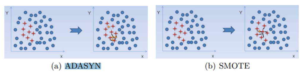
Fig. 2 Difference between ADASYN and SMOTE algorithms (Letteri et al., 2020, p. 7)
It generates minority data samples according to their distributions. Thus, more minority class samples are generated that learn hardly as compared to those minority samples that are easier to learn. The ADASYN method can not only reduce the learning bias introduced by the original imbalance data distribution but can also adaptively shift the decision boundary to focus on those difficult to learn sample (He et al., 2008, pp. 1323).
K-Means SMOTE Oversampling
K-Means SMOTE works in three steps:
- Cluster the entire input space using k-means.
- Distribute samples to:
- Select clusters which have a high number of minority class samples.
- Assign more synthetic samples to clusters where minority class samples are sparsely distributed.
- Oversample each filtered cluster using SMOTE.
The method implements SMOTE and random oversampling as limit cases (kmeans-smote.readthedocs.io, n.d.).
Undersampling
Cluster Centroids
It reduces the majority class by replacing a cluster of majority samples by the cluster centroid of a KMeans algorithm. This algorithm keeps N majority samples by fitting the KMeans algorithm with N cluster to the majority class and using the coordinates of the N cluster centroids as the new majority samples (imbalanced learn, n.d., b).
Condensed Nearest Neighbour
Condensed Nearest Neighbor reduces the dataset for k-NN classification by using a subset of examples (Gowda and Krishna, 1979, pp.488). Nearest neighbor rule decides how to remove a sample or not. The algorithm is runs as given below:
- Get all minority samples in a set.
- Add a sample from the targeted class.
- Classify each sample using nearest neighbor rule.
- Add a sample if it is misclassified.
- Repeat the procedure until there are no samples to be added.
(imbalanced learn, n.d. f)
Edited Nearest Neighbor
This method cleans dataset by removing samples close to the decision boundary (imbalanced learn, n.d., c).
Samples are classified using nearest neighbor rule and then classified using single nearest neighbor rule of the pre-classified samples (Wilson, 1972, pp.408).
Repeated Edited Nearest Neighbor
This repeats the Edited Nearest Neighbor many times (imbalanced learn, n.d., d).
AIIKNN
This method applies Edited Nearest Neighbor several times and will vary the number of nearest neighbours (imbalanced learn, n.d. e). AIIKNN differs from the previous Repeated Nearest Neighbor as the number of neighbors of the internal nearest neighbors algorithm is increased at each iteration (imbalanced learn, n.d. e).
Instance Hardness Threshold
Samples of the class with low probabilities are removed from the dataset. Sampling strategy is based on the result. If the result is float, then it is the ratio of majority to minority class. There is a problem of class overlap (imbalanced learn, n.d. f; Sisters, 2020).
NearMiss Undersampling Technique
This method randomly eliminates samples from the larger class. When two points belonging to different classes are very close to each other in the distribution, this algorithm eliminates the samples of the larger class to balance the distribution. The steps taken by this algorithm are:
- Calculates the distance between all the points in the larger class and compares them with the points in the smaller class.
- Samples of the larger class that have the shortest distance with the smaller class are selected. These n classes need to be stored for elimination.
- If there are m instances of the smaller class, then the algorithm will return m*n instances of the larger class.
(Madhukar, 2020)
Tomek Links
Tomek Links is a modification from Condensed Nearest Neighbors. CNN method only randomly selects the samples with its k nearest neighbors from the majority class that are removed. Tomek Links method uses the rule to selects the pair of observation (a and b) that are fulfilled these properties:
- The observation a’s nearest neighbor is b.
- The observation b’s nearest neighbor is a.
- Observations a and b belong to a different class. That is, a and b belong to the minority and majority class vice versa.
(Viadinugroho, 2021)
Neighbourhood Cleaning Rule Undersampler
This class uses Edited Nearest Neighbor and a k-NN to remove irrelevant samples from the datasets (imbalanced learn, n.d. g). Neighborhood Cleaning Rule (NCL) is an undersampling method to overcome imbalance class distribution by reducing the data based on cleaning. Cleaning process is improvised by removing the three closest neighbors from the data which are incorrectly classified. The data cleaning process is for both majority and minority class. Basically, the principle of NCL is based on the concept of One-Sided Selection (OSS), which is one technique for reducing data based on the instances to reduce classes carefully. (Agustianto and Destarianto, 2019, pp. 87)
Hybrid Sampling: Oversampling combined with Undersampling
This method can generate noisy samples which is solved by cleaning the space resulting from over-sampling. After SMOTE over-sampling, Tomek’s link and edited nearest-neighbours are the two cleaning methods are applied to the pipeline.The two ready-to use classes imbalanced-learn implements for combining over- and undersampling methods are: (i) SMOTETomek and (ii) SMOTEENN (imbalanced learn, n.d. h)
Stratified k-fold Cross Validation
Stratified k-fold cross-validation is a technique used in machine learning for model evaluation and hyperparameter tuning. It is particularly useful when dealing with imbalanced datasets, where the distribution of classes is uneven. The method involves dividing the dataset into k-folds while ensuring that each fold maintains the same class distribution as the original dataset. This helps to mitigate the risk of bias in model evaluation by ensuring that each class is adequately represented in both the training and testing subset
- The dataset is first divided into k equal-sized folds.
- For each fold, the class distribution is preserved, meaning that each fold contains approximately the same proportion of each class as the original dataset.
- The model is trained on k-1 folds and evaluated on the remaining fold
- This process is repeated k times, with each fold serving as the validation set exactly once
- The final performance metric is computed by averaging the performance across all k folds
Stratified k-fold cross-validation helps to produce more reliable estimates of model performance, especially in scenarios where the class distribution is skewed (Kojavi, 1995).
Evaluation Metrics
Confusion Matrix
In a confusion matrix, columns correspond to the predicted class, while rows correspond to the actual class. The components of the matrix are as follows:
- True Negatives (TN): The count of negative examples that are correctly classified as negative.
- False Positives (FP): The count of negative examples that are incorrectly classified as positive.
- False Negatives (FN): The count of positive examples that are incorrectly classified as negative.
- True Positives (TP): The count of positive examples that are correctly classified as positive.
Evaluation metrics used in image identification are typically accuracy, precision, recall, F1- score (Al-Sarayreh et al., 2018; Larsen et al., 2014; Ropodi et al., 2015; Setyono et al., 2018; Wang et al., 2019).
Accuracy
Accuracy and F1 scores are described in Eq. 1 and 2 respectively (Prakash et. al., 2021)
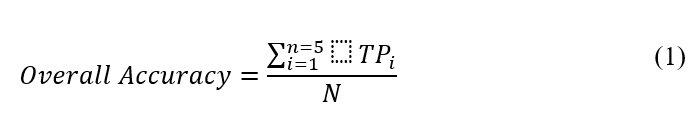
In Eq. 1, TPi or the true positive is the number of instances predicted correctly for instance and
is the total number of predictions.
F1 Score
where,
Precision
(Prakash el. al., 2021)
Precision
Precision is defined as the ratio of true positive defects correctly detected to the total number of detected defects (Peng et al., 2020, p. 7). Precision indicates how effectively a model identifies true positives, ensuring that the positive detections are accurate (Chawla, V. N. et al., 2002, p. 326).
Recall
Recall, often referred to as sensitivity or true positive rate, is the ratio of correctly detected true defects (true positives) to the total number of true defects (Peng et al., 2020, p. 7). Recall showcases the model’s capacity to identify all positive instances, thus assessing its ability to capture all actual positives (Chawla, V. N. et al., 2002, p. 326).
The F-value, also known as the F-score or F-measure, represents the harmonic average of precision and recall (Minhas and Zelek, 2020, p. 510; Zhao et al., 2020, p. 23).
The F-value combines both recall and precision, and it reaches its highest value when both recall and precision are high (Han et al., 2005, p. 880).
For imbalanced datasets, accuracy can be misleading. Even if a classifier correctly classifies all majority examples but misclassifies all minority examples, the high accuracy results from the significant number of majority examples. This renders accuracy unreliable for predicting the minority class (Han et al., 2005, p. 879).
For balanced datasets, the error rate is utilized as a performance metric:
Error Rate = 1 – Accuracy (Chawla, V. N. et al., 2002, p. 322)
In imbalanced datasets, the error rate isn’t an appropriate performance measure. Instead, precision and recall are more meaningful metrics (Chawla, V. N. et al., 2002, p. 326).
Tensorflow and Keras
Tensorflow is an open source machine learning framework designed for building and training of machine learning models and neural networks. It consists of libraries and tools for machine learning tasks (Tensorflow, n.d.).
Keras is an open-source neural network library written in Python. It is designed to be user-friendly, modular, and extensible, allowing users to quickly prototype and build deep learning models with minimal code. Keras was originally developed by François Chollet and was integrated into TensorFlow as its official high-level API starting from TensorFlow version 2.0. Keras provides a simple and intuitive API that allows users to define neural networks using high-level building blocks like layers, activations, optimizers, and loss functions. Keras supports both convolutional and recurrent neural networks, as well as combinations of the two. It also provides support for various types of layers, such as dense, convolutional, recurrent, and more (Chollet et al., 2015).
Data Visualization
Principal Component Analysis
It is a statistical method to reduce the dimensionality of a dataset. It determines the direction where the variation in the dataset is maximum. This direction is called the “principal component”. It determines the different principal components (directions) within the dataset and then uses these principal components to represent the samples. In this way samples can be plotted to check the similarities or differences between the samples. This enables to group the samples. Principal components are the linear combinations (new variables) of the original variables (Ringner, 2008, pp. 303). PCA is a technique for feature extraction. It combines all the variables and then drops less important variables. In this way new independent variables are created. It identifies the relationships between variables and then determines direction of dispersion in the dataset (Brems, 2017).
Visual Studio Code
Visual Studio Code (VS Code) is a free, open-source code editor developed by Microsoft. It is widely used by developers for writing and debugging code, and it supports a wide range of programming languages and frameworks. Here are some key features and aspects of Visual Studio Code. While it is technically a code editor, VS Code offers many features commonly found in integrated development environments (IDEs) (Microsoft, n.d.).
Research Question
The objective of this research is to address the following research questions:
- Is it feasible to create a deep learning methodology for fabric defect detection that combines
- efficient speed,
- heightened accuracy and
- comprehensive training encompassing various fabric defect types.
- Can this method incorporate a balanced approach to minimize false negatives in detection rates?
The focus was placed on deep learning algorithms. While a considerable amount of research has been done, several limitations persist, and a system that meets the criteria for deployment within industry has not been achieved.
Materials and Methods
Dataset
The data collected for this project were from [3] [4] :
- Fabric Defect Dataset from Kaggle (Ranathunga, 2020)
- Fabric Stain Dataset from Kaggle (Pathirana, 2020).
- Aitex fabric image database (Silvestre-Blanes et al., 2019)
- Dataset from the author of the literature review paper (Peng, 2020): only the non-defect images from the dataset.
Aitex fabric image database
This textile fabric dataset consisted of 245 images of 7 different fabrics with image sizes of 4096×256 pixels. There were 140 defect-free images, 20 for each type of fabric. In each of the defected category, there were 105 images (Silvestre-Blanes et al., 2019).
Fabric Stain Dataset
This was taken from Kaggle (Pathirana, 2020). The dataset was built as a part of the fabric defect detection project of the Intelligence Lab of University of Moratuwa, Sri Lanka. The dataset consisted of images with resolution of 1920×1080 or 1080×1920. It consisted of 398 defected images with different types of stains and 68 defect free images.
Fabric Defect Dataset
The dataset was also taken from Kaggle and it was supplied by the Intelligence Lab, Department of computer science and Engineering, University of Moratuwa (Ranathunga, 2020). This dataset consisted of 3 classes of defective images namely horizontal, vertical and holes along with 3 mask images for each defective image sample. The folder named ‘captured’ consisted of raw images. Images have a size of 640×360.
Dataset from the author of the literature review paper
Authors of the research papers in the literature review were contacted through emails for the dataset. With the consent of the author of the paper “Automatic fabric defect detection method using pran-net” (Peng, 2020) named Troy Peng, the annotated data was used (Peng et. al, 2020).
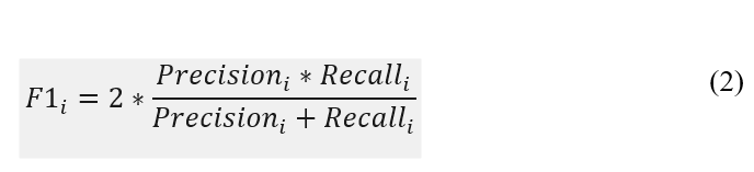
After collecting the images from all these sources, the distribution of the images is as given below:
- Defect free 1,666
- Defected 1,073
Defected hole 281
Defected horizontal 136
Defected lines images 157
Defected stain images 398
Defected verticle images 101
Fig. 3 Number of images in each class of the dataset
Total Images = 2,739
Experimental Setup and Evaluation
The images were experimented with two distinct sizes:
- 150×700
- 245×345
The entire experiment was carried out using the Python programming language [5] [6] . Keras [7] [8] , in conjunction with TensorFlow [9] [10] , was employed for the development and training of CNN. Various libraries, including numpy, pandas, and scikit-learn, were used for supporting tasks. The experimentation was conducted within the Visual Studio Code (VS Code) [11] [12] [13] environment.
Data Pre-processing
The acquired dataset exhibited an imbalance in its distribution across different classes. Consequently, various sampling techniques from the imbalanced-learn module were applied and tested on the three chosen image sizes i.e. 150×700, and 245×345. The objective was to determine the most effective sampling technique that yields high performance.
Data Visualization
Data visualisation was facilitated through Principal Component Analysis (PCA).
Principal Component Analysis (PCA) is considered good for data visualization for several reasons:
- PCA reduces the number of dimensions in the data while preserving as much variance as possible. This simplifies complex datasets and makes them easier to visualize, typically in 2D or 3D.
- By projecting data onto principal components that capture the most variance, PCA highlights the underlying structure and patterns, making relationships in the data more apparent.
- PCA can help in removing noise and redundant information, which can clarify the visual representation of the data
Modelling- Convolutional Neural Network
A CNN model’s architecture was designed to facilitate multi-classification and consisted of five two-dimensional convolutional layers for feature extraction.
- The initial convolutional layer was configured with 16 filters, each having a 7×7 kernel size. The second convolutional layer used a set of 32 filters with a 5×5 kernel size.
- The third layer used 64 filters with a 3×3 kernel size.
- The fourth layer comprised 128 filters with a kernel size of 3×3.
- Lastly, the fifth layer was equipped with 256 filters and used a 3×3 kernel size.
Padding with the hyperparameter ‘same’ was applied to allow the filter kernels to traverse the images by including additional pixels. Using ‘same’ as the padding hyperparameter ensured that the size of the output feature map remained the same as that of the input feature map.
Each successive convolutional layer was accompanied by batch normalization, an activation function, max pooling, and dropout layers. Batch normalization was used to standardize and normalize the dataset within batches, contributing to improved training and learning speed.
The outputs of linear operations, such as convolutions, passed through nonlinear activation function Rectified Linear Unit (ReLU). Rectified Linear Unit (ReLU) activation function was employed due to the multi-layered nature of the CNN.
For this novel model, Max pooling was adopted to reduce image dimensions and achieve downsampling, creating lower-resolution images with essential features. A 2×2 filter shape was employed for max pooling since it should be smaller than the feature map’s dimensions. This pooling layer generated new feature maps. Dropout layers were introduced to address overfitting.
In the final phase of the model, a fully connected layer, also known as a dense layer, was used to align the outputs from the pooling layers with the dataset labels. Since multiple pooling layers were employed, a flattening layer was introduced to organize these outputs sequentially into a vector. After passing through all the convolutional layers, the output took the form of a multidimensional array, which was then fed into a dense layer. To interpret the results as a probability distribution, a SoftMax function was applied in the fully connected layer.
To evaluate compatibility between network output predictions and given labels, a loss function i.e. Adaptive Moment (Adam) function was employed.
Parameter Settings
For this novel idea, for each experiment, the dataset was divided into a training set and a test set using a 95:05 stratified sampling ratio. The validation data was used to examine if the hyperparameters required further tuning. The test data was used as an unseen dataset to examine the results of the model. The training process encompassed 100 epochs , with a batch size of 6 samples per batch.
Using a stratified k-fold cross-validation approach with 10 folds, the dataset is split into training and validation sets for each fold. For every fold iteration, a Convolutional Neural Network (CNN) model is created using the specified image shape and trained on the training data for 100 epochs with a batch size of 6. The model’s performance is evaluated on the validation set, and both the validation loss and accuracy are recorded. This iterative process allows for a comprehensive assessment of the model’s performance across multiple folds, contributing to a more reliable evaluation of its generalization capabilities.”
Evaluation Metrics
Evaluation metrics used were accuracy, precision, recall, F1- score, confusion matrix.
Validation Time
This is the time taken to evaluate the performance of the model on the validation dataset after each epoch (or at specified intervals during training). The validation dataset is a separate set of data not used for training but for assessing how well the model is generalizing. This helps in tuning the model’s hyperparameters and prevents overfitting. The validation time includes the time required to compute metrics like accuracy, precision, recall, and F1 score on this dataset
Modelling Time
Also known as training time, this is the duration required for the model to learn from the training dataset. It includes the time taken for forward and backward propagation through the network for all epochs until the model converges. This phase involves the optimization of the model parameters (weights and biases) through iterative updates. Efficient modeling time is critical for developing models quickly, especially when dealing with large datasets or complex architectures
Prediction Time
This is the time it takes for the trained CNN model to make predictions on new, unseen data. It measures how quickly the model can infer the class labels or other outputs for input data during deployment. Low prediction time is essential for real-time applications, where the model needs to provide results almost instantaneously, such as in autonomous driving or live video analysis.
Results
CNN Modelling was performed for the two selected sizes of images dataset without any sampling technique. In order to optimize the performance of the CNN model, sampling techniques available in the imbalanced-learn module were experimented to select the best sampling technique with high performance. The results were as given in table 1, 2 and 3.
| Parameters | |||
| Total | Trainable | Non-trainable | |
| 245×345 | 2,698,310 | 2,697,062 | 1,248 |
| 150×700 | 3,157,062 | 3,155,814 | 1,248 |
Table 1 Total number of trainable and non-trainable parameters for the two image sizes
Table 2 Model performance without and with data pre-processing
| 245×345 | 150×700 | |||||
| Validation Time | Model Time | Pred Time | Validation Time | Model Time | Pred Time | |
| Sec | Sec | Sec | Sec | Sec | Sec | |
| Without Sampling | 2.64 | 0.22 | 0.06 | 3.26 | 0.34 | 0.06-0.1 |
| Undersampling | ||||||
| ClusterCentroids | 2.8 | 0.29 | 0.06-0.1 | 3.11 | 0.205 | 0.07-0.08 |
| AllKNN | 2.69 | 0.21 | 0.07 | 3.52 | 0.24 | 0.07-0.08 |
| Condensed Nearest Neigbor | 2.52 | 0.2 | 0.07 | 3.18 | 0.20 | 0.06-0.15 |
| Edited Nearest Neighbour | 2.5 | 0.2 | 0.09 | 3.3 | 0.22 | 0.09 |
| Repeated Edited Nearest Neighbout | 2.6 | 0.2 | 0.06 | 3,12 | 0.21 | 0.05-0.7 |
| Instance Hardness Threshold | 2.50 | 0.21 | 0.07 | 3.32 | 0.2 | 0.08 |
| Near Miss | 2.69 | 0.24 | 0.07 | 3.2 | 0.2 | 0.07 |
| Neighbourhood Cleaning Rule | 2.82 | 0.24 | 0.07 | 3.4 | 0.25 | 0.06-0.14 |
| TomekLinks | 2.45 | 0.27 | 0.06-0.1 | 2.93 | 0.3 | 0.08-0.1 |
| Random Undersampler | 2.55 | 0.23 | 0.06-0.08 | 3.86 | 2.51 | 0.09 |
| Oversampling | ||||||
| ADASYN | 2.43 | 0.56 | 0.08-0.1 | 3.53 | 0.89 | 0.08 |
| Random Oversampling | 2.90 | 0.7 | 0.06-0.1 | 2.98 | 0.23 | 0.07 |
| Borderline SMOTE | 3.25 | 1.96 | 0.06-0.096 | 3.31 | 1.74 | 0.087-0.065 |
| kMeans SMOTE | 3.2 | 1.1 | 0.09 | 3.47 | 5.66 | 0.077 |
| SMOTEN | 3 | 1.9 | 0.07 | 3.36 | 2.02 | 0.07-0.09 |
| SMOTENC | ||||||
| SVM SMOTE | 3.15 | 1.90 | 0.085-0.1 | 3.40 | 1.86 | 0.07-0.086 |
| Combined Oversampling and Undersampling | ||||||
| SMOTEENN | 3,4 | 1.57 | 0.09 | 3.5 | 1.15 | 0.07-0.1 |
| SMOTETomek | 2.77 | 2.21 | 0.06 | 3.67 | 2.44 | 0.07-0.12 |
| Ensemble | ||||||
| Pipeline (AIKNN+Neighbouhood CleaningRule) | 2.8 | 0.31 | 0.07 | 3.26 | 0.35 | 0.06-0.09 |
| Miscellaneous | ||||||
| Function Sampling | 2.59 | 0.21 | 0.07-0.1 | 3.26 | 0.2 | 0.07-0.15 |
Table 3 Model time performance with data pre-processing
Discussion
The aims of this study were twofold: to amass an image dataset containing fabric defects and to create a model capable of accurately categorizing these defects, ultimately leading to an automated system for identifying and detecting fabric defects.
To do this, state-of-the-art data sampling techniques were applied to the dataset consisting of a total of 2,739 images, including a total of 1666 non-defected images and 1,073 defected images. These sampling techniques were experimented on a novel CNN image detection methodology. These results demonstrated some interesting findings relating to AI and implementation strategies for future commercial deployment strategies.
As depicted in table 2, when analyzing the dataset without pre-processing, the CNN model’s performance was impacted by the imbalanced nature of the data. For images size 150 x 700, the model achieved 91% accuracy, precision, recall, and F1 score, respectively. However, with images sized 245×345, the model’s performance notably improved, reaching 94% accuracy, 96% precision, 94% recall and F1 score. Remarkably, the 245×345 image size demonstrated superior performance compared to the larger 150×700 image size. But even then, the performance was not outstanding and needed further improvement. For this reason, different sampling techniques were experimented to improve the performance of the model.
Oversampling
In table 2, it is evident that ADASYN, Random Oversampling, Borderline SMOTE, and SVM SMOTE yielded superior performance when applied to images sized 245×345 compared to those sized 150×700, across metrics such as accuracy, precision, recall, and F1 score. Unfortunately, SMOTENC encountered memory size limitations and could not be executed. Notably, kMeans SMOTE and SMOTEN did not exhibit enhanced performance.
Among the oversampling techniques, Random Oversampling, Borderline SMOTE, and SVM SMOTE showcased exceptional performance. Notably, Random Oversampling achieved a precision of 97%, outperforming the other techniques in this regard.
As indicated in Table 2, both Random Oversampling and ADASYN exhibited notably quicker validation and modeling times for images sized 245×345 compared to other oversampling methods, as well as compared to the 150×700 size across all methods. The longest validation times were observed for kMeans SMOTE, Borderline SMOTE, SMOTEN, and SVM SMOTE.
Undersampling
None of the undersampling techniques demonstrated satisfactory performance for either of the two image sizes. However, Neighbourhood Cleaning Rule and AIIKNN showcased notable improvements. Neighbourhood Cleaning Rule exhibited superior performance, achieving 95% across accuracy, precision, recall, and F1 Score for images sized 245×345. AIIKNN displayed enhanced precision, reaching 97% and 95% for images sized 245×345 and 150×700, respectively.
The validation, modeling, and prediction times for both AIIKNN and Neighbourhood Cleaning Rule were nearly equivalent to the model’s performance without sampling. This held true for both image sizes, 245×345 and 150×700. Among the undersampling techniques, Tomeklinks exhibited the shortest validation, modeling, and prediction times.
Combined Undersampling and Oversampling
Remarkably, both SMOTEENN and SMOTE Tomek surpassed the performance of combined oversampling and undersampling techniques. Particularly, SMOTEENN demonstrated superior performance compared to SMOTE Tomek.
Ensemble
As depicted in Table 2, the Pipeline sampling utilized undersampling techniques AIKNN and Neighbourhood Cleaning Rule. Due to limited memory space, oversampling techniques could not be evaluated. Consequently, the Pipeline could not demonstrate any performance across both image sizes.
Miscellaneous
The Function sampler did not exhibit any performance improvement with the image size 245×345. However, for the larger image size of 150×700, performance was notably better, with 96% accuracy, recall, and F1 score, and 97% precision.
From Table 2, it’s apparent that among the best-performing sampling techniques across various experimented methods, SMOTEENN, combining oversampling and undersampling, delivered the most promising performance compared to other selected top-performing methods. The CNN model’s performance with the SMOTEENN sampling technique was notably strong for the image size of 245×345.
The following table (Table 4) provides an overview of the best-performing techniques among the different sampling methods tested with two image sizes: 150×700 and 245×345. As shown in the table, the combined oversampling and undersampling techniques yielded the best results. Among the two combined techniques tested, SMOTEENN and SMOTETomek, SMOTEENN achieved the highest performance with 98% accuracy, precision, recall, and F1 score for the 245×345 image size.
For SMOTEENN, the validation, modeling, and prediction times for the 245×345 image size were nearly the same as for the 150×700 image size. However, for SMOTETomek, the validation time for the 245×345 size was lower (2.7 seconds) compared to SMOTEENN (3.4 seconds). Conversely, the modeling time for SMOTETomek was higher (2.21 seconds) compared to SMOTEENN (1.57 seconds).
The performance of SVM SMOTE, Random Oversampling, and Borderline SMOTE—techniques categorized under oversampling for the 245×345 image size—and the miscellaneous sampling technique, Function Sampler, for the 150×700 image size, remained nearly identical in terms of accuracy, precision, recall, and F1 score. The validation, prediction, and modeling times for SVM SMOTE, Random Oversampling, and Borderline SMOTE were relatively shorter compared to the combined oversampling and undersampling technique, SMOTEENN.
For images sized 245×345, the validation, modeling, and prediction time for SMOTEENN was longer compared to SMOTE Tomek, being the maximum among the undersampling and oversampling techniques. SMOTE Tomek exhibited shorter validation times, outperforming other undersampling and oversampling techniques. However, as SMOTEENN has surpassed SMOTETomek in terms of accuracy and precision, therefore, SMOTEENN remains on the top of SMOTETomek and among other sampling techniques in terms of overall performance.
Table 4 Performance comparison of the best performing sampling techniques
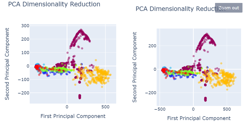
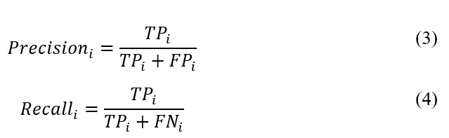
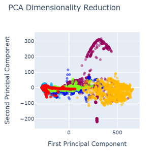
When analysing results, PCA was used for the data visualization. Figure 4 shows the data set before data preprocessing.
Fig. 4 PCA before data pre-processing
- Red colored narrates the defect free images.
Defected images are shown as:
- Royal Blue shows the holes,
- Orange shows vertical
- Green shows lines
- Light blue shows horizontal
- Yellow shows stains
As shown in the figure 4, defects are not properly segregated and therefore, model could not predict the defect classes accurately and precisely.
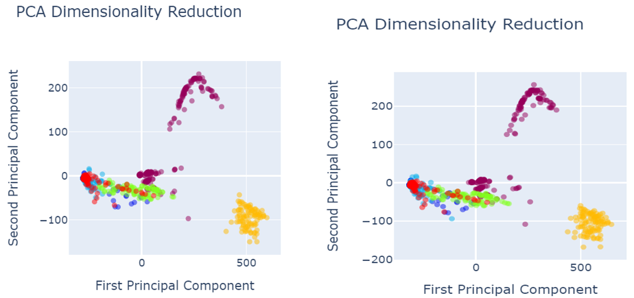
The following figures give the data visualization using Principal Component Analysis for the best performing techniques given in the table. For example, the yellow dots representing stains could be misclassified as defect-free since they are mixed with the red dots. Similarly, the royal blue dots are mixed with the green dots, leading to potential misclassification of defects. A similar issue occurs with the royal blue dots, which are mixed with the green dots, leading to potential misclassification of these defects.
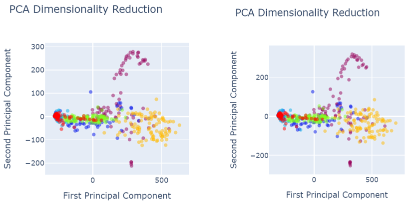
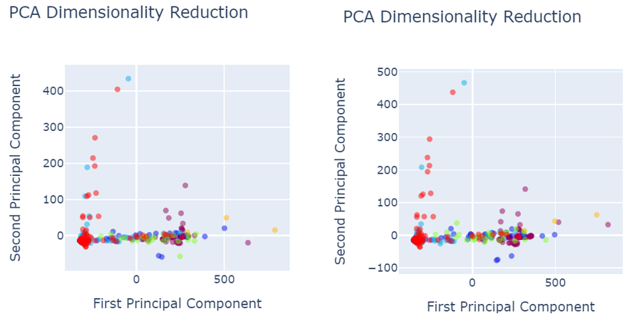
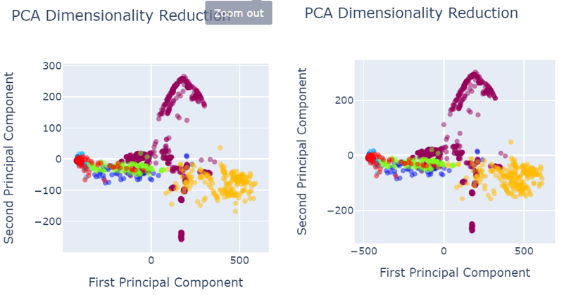
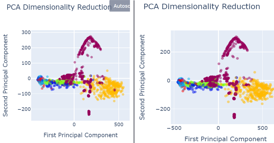
Fig. 5 shows the data visualization when data was pre-processed using best performed sampling techniques.
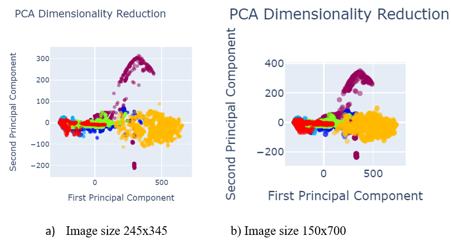
- Image size 245×345 b) Image size 150×700
Fig. 5 PCA after data pre-processing with SMOTEENN sampling technique
a
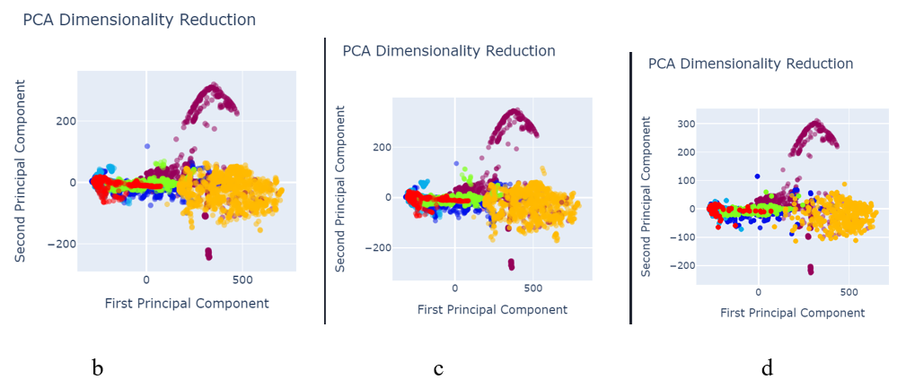
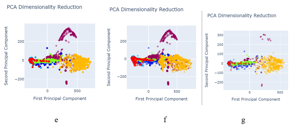
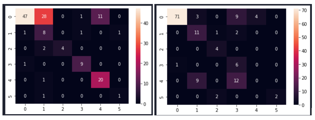
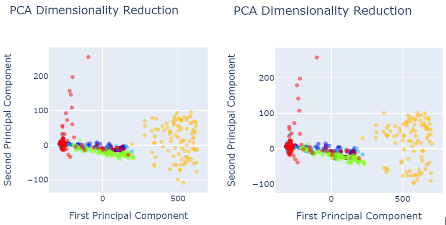
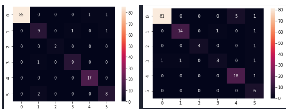
Fig. 6 PCA after data pre-processing with:
a) SMOTETomek image size 245×345
b) SVM SMOTE Oversampling image size 245×345
c) SVM SMOTE Oversampling image size 150×700
d) Random Oversampling image size 245×345
e) Random Oversampling image size 150×700
f) Borderline SMOTE image size 245×345
g) Function Sampler image size 150×700
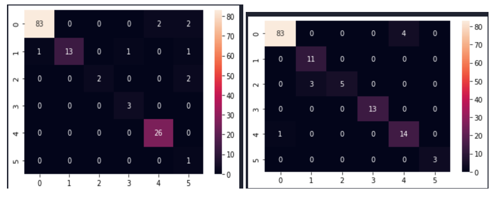
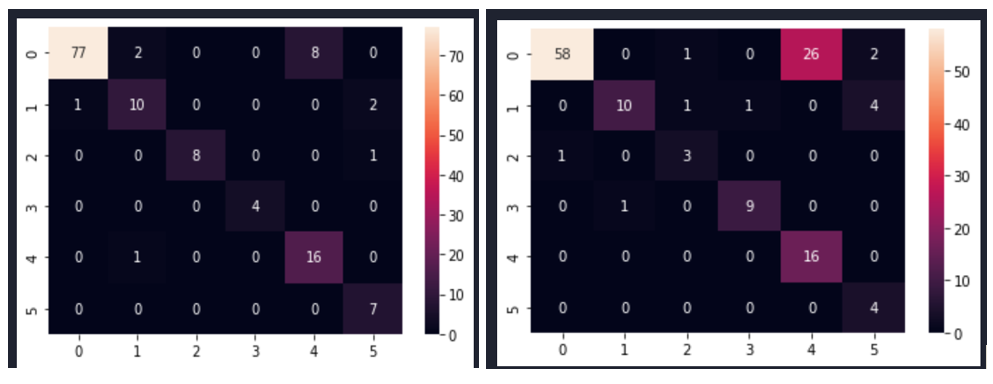
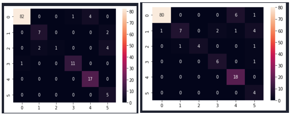
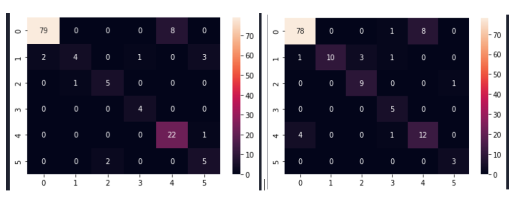
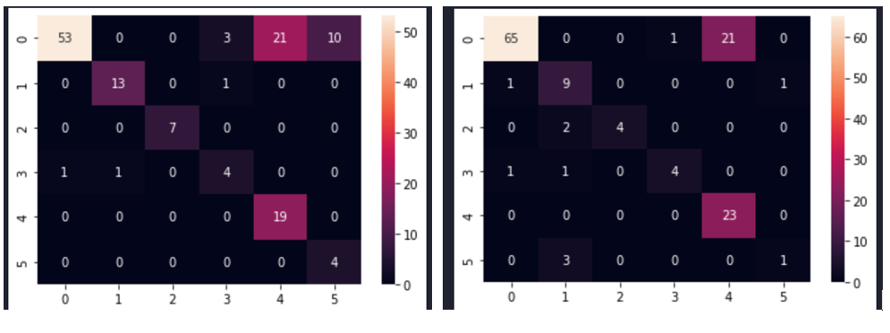
Fig. 7 shows the confusion matrices after modelling with CNN for the selected size 245×345.
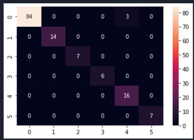
Fig. 7 Confusion matrix of the CNN model sampled with SMOTEENN method for image size 245×345
a)Image size 245×345
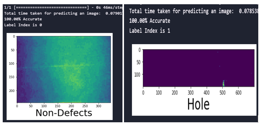
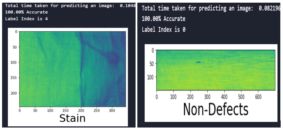
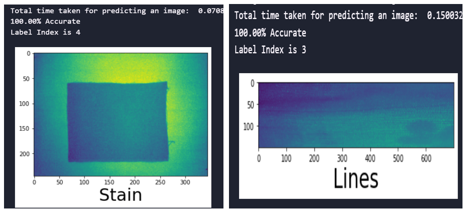
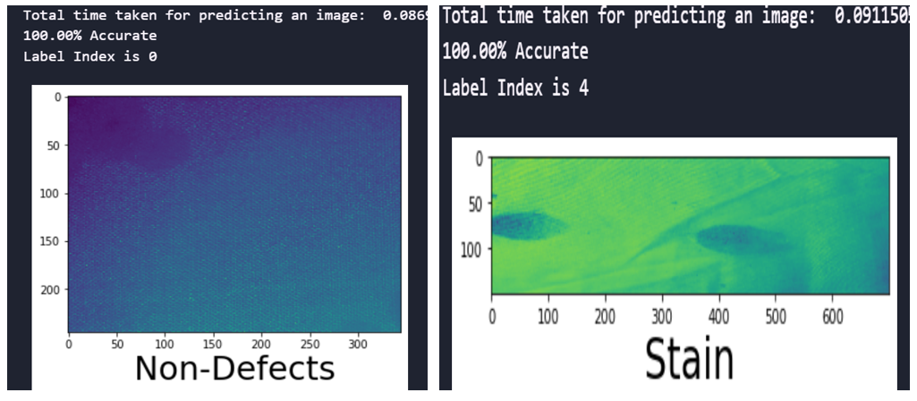
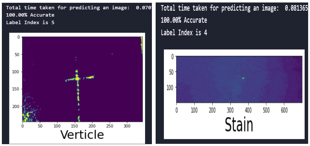
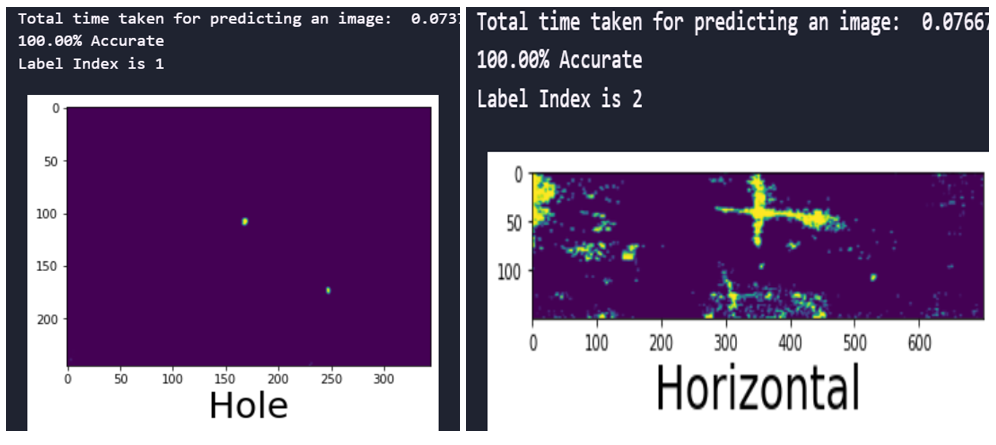
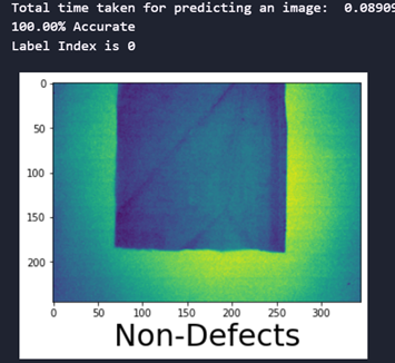
Fig. 8 Prediction time and accuracy of the CNN model with SMOTEENN sampling technique
fig.8 shows the time taken and accuracy for predicting the defects and the accuracy of predictions for the developed CNN with SMOTEENN sampling techniques for the image size 245×345. It is evident that the trained model performance remained 100% accurate.
Verification from Literature Review
The findings from the experimentation align with the conclusions drawn by Luke, Joseph, and Balaji (2019, p. 70), which are elaborated below:
- CNN significantly influences image resolution accuracy.
- Image sizes exert a substantial impact on model accuracy. Changes in size can either enhance or degrade model performance.
- Accuracy tends to increase as image sizes are enlarged, but this trend reverses beyond a certain threshold due to reduced receptive field.
- Larger image sizes impact the ability to learn medium and high-level features.
- To achieve higher accuracy, the optimal image size falls within the range between the default size and 512.
- Resizing images affects low-level features due to information loss, thereby influencing accuracy. The accuracy is particularly influenced by inter-class similarities, which are closely tied to low-level features (Luke, Joseph, and Balaji, 2019, p. 79).
Image resolution notably influences the model’s performance. Thambawita et al. (2021) discovered that CNN achieved its best performance with a larger image size of 512×512 compared to 32×32 (Thambawita, et al., 2021).
Horwath et al. (2020, p. 4) noted that image segmentation becomes challenging with high-resolution images due to issues recognizing interface pixels without considering the background. The complexity of features increases accordingly.
Sabottke and Spieler (2020, p.2) emphasized that a lower number of parameters leads to improved model performance by reducing overfitting risk. However, excessive resolution reduction may result in a loss of valuable information. They found that CNN performance was optimal within the range of resolutions between 256×256 and 448×448 image sizes. Their conclusion was that there’s a trade-off between increasing image resolution and the maximum feasible batch size. A high number of parameters affects model performance not solely due to overfitting but also because of the intricacies involved in optimization (Sabottke and Spieler, 2020, p. 2).
Rukundo (2021, p. 17) highlighted that determining the optimal image size for training datasets is a significant challenge. He observed that a size of 256×256 outperformed 128×128, attributing this improvement to the lower cross-entropy loss in a U-net trained on a 256×256 training image set. He emphasized that lower loss corresponds to greater model accuracy.
Result comparison with models from the related works
Until today, fabric defect detection tasks have primarily been carried out manually. Numerous research studies have proposed defect detection algorithms; however, these methods have certain limitations. They often suffer from slow processing speeds and lack the capability to effectively detect a wide range of defect types. Consequently, these methods have not found practical applicability within the textile industry.
The following table gives a brief view of the evaluation of the models discussed in the section of related works.
| Accuracy % | Precision % | Recall % | F1 Score % | Detection Time | |
| Peng et. al (2020) PRAN-NET Denim | 91.99 | 9.7 Frame per sec | |||
| Peng et. al (2020) PRAN-NET Plain | 98.66 | 25.4 Frame per sec | |||
| Almeida, Moutinho and Matos-Carvalho (2021) CNN-FN Reduction | 75.45 | 72.76 | 88.47 | 5.69 ms per image | |
| Zhao et. al (2019) CNN-VLSTM | 95.73-99.47 | 95.74-100 | 95.73-100 | 95.73-100 | 1.8-3.5 e2 |
| Wei et. al (2019) Faster RCNN | 95.88 | 0.3 sec | |||
| Liu et al. (2019) VGG16 | 97.7 | ||||
| Liu et al. (2019) LZFNet | 98 | 13.8 ms | |||
| Cheng et al. (2022) SCUNet | 98.01 | 96.86 | |||
| Our Model 99 100 99 99 0.06-0.07 sec | 98 | 98 | 98 | 98 | 0.06-0.07 sec |
Table 5 Performance comparison of different models from the literature review with our model
All the models discussed in the related works section exhibited a common drawback: they are slow and time-consuming, rendering them unsuitable for various types of fabric defects. Although CNNs based on visual VLSTM presented by Zhao et al. (2019) demonstrated superior performance in terms of accuracy and speed but they also exhibit significant sensitivity to intricate fabric structures.
The performance of the model developed by Zhao et al. (2019) is given in the table 8.
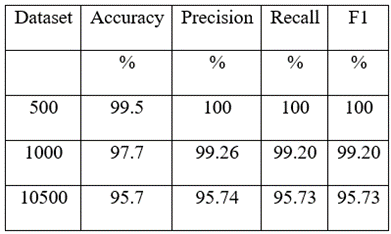
Table 6 Performance metrics of Zhao et al. (2019) model
The model developed by Zhao et al. (2019) was based on visual long-short term memory (VLSTM). In contrast to the model proposed by Zhao et al. (2019), the current model is:
- notably simpler,
- lacking the integration of the CNN architecture with other mechanisms.
- Zhao et al. (2019) conducted experiments with varying image quantities, such as 500, 1000, and 10500, and identified the dataset consisting of only 500 images as yielding the best performance. However, the performance of the larger image datasets, particularly the 1000-image dataset, was suboptimal.
In contrast, the CNN model devised in this research exhibited superior performance when trained with a substantial dataset comprising 2,739 images, particularly excelling with the image size of 245×345. Consequently, the model discussed in this research paper emerges as the most suitable candidate for deployment within the textile industry.
The SCUNet model, developed by Cheng et al. (2022), exhibits several limitations. Notably, the experimentation involved a singular image size of 256×256, a small dataset comprising only 106 grayscale images, and data processing utilizing image cropping and augmentation. Importantly, the model’s performance on colored data images remains unknown, as the experiments focused solely on grayscale images. Cheng et al. (2022, p. 3115) acknowledge a limitation wherein the model requires fabric to be “flat”; however, the term is inaccurately used, as the authors seem to refer to “plain” fabric—fabric devoid of patterns or designs. The model’s inadequacy in handling designed fabrics is evident. Cheng et al. (2022, p. 3117) claim time efficiency compared to manual visual inspection but fail to present metrics for detection time, leaving the efficiency and speed of defect detection unmeasured. In contrast, our research paper not only addresses detection time but also evaluates the model’s efficiency. Our model, tested on both colored and grayscale images, encompasses all defect sizes. The dataset, curated from various sources, includes plain and patterned fabrics. In direct comparison, our model outperforms SCUNet with an overall accuracy of 98% and recall of 98%. This achievement is particularly noteworthy given our comprehensive experimentation with diverse fabric types, defect sizes, and image variations, demonstrating superior adaptability and performance.
Conclusion
This research introduces an innovative approach for the automated detection of fabric defects within the textile industry. Within this sector, the journey begins with yarn from the spinning department, which is then utilized in the weaving unit to create greige fabric. The subsequent stages involve processes such as scouring, bleaching, dyeing, and finishing the fabric. Once the fabric reaches the finished state, it undergoes a quality assessment before proceeding to the stitching department for garment production. During the quality inspection phase, the fabric is placed across quality tables, where inspectors meticulously examine it and identify any instances of fabric defects, marking the fabric as necessary.
The objective of this study was to identify a suitable deep learning algorithm capable of automating fabric quality inspection in the textile industry, thereby replacing the labor-intensive manual process. After conducting a comprehensive literature review, a convolutional neural network (CNN) algorithm was chosen as the basis for the research. To determine the optimal image size for the algorithm, two sizes—150×700, and 245×345—were tested to achieve the best model performance. Addressing the challenge of dataset imbalance, various sampling techniques were employed and evaluated.
Remarkably, the research revealed that the CNN model yielded the most impressive results when combined with the SMOTEENN sampling technique. This outcome signifies a significant advancement in automating fabric quality inspection within the textile industry.
The research highlighted the substantial impact of image size on the model’s performance. The CNN model that was developed demonstrated its most exceptional performance when paired with the SMOTEENN sampling technique. Among the two tested image sizes—150×700, and 245×345—the 245×345 size emerged as the most optimal performer.
In terms of practical application, this model stood out for its swift processing times. Specifically, for the image sizes 245×345, the model achieved a validation time of just 3.4 seconds and a prediction time of 0.09 seconds. While the 150×700 size demanded 3.5 seconds and 1.15 seconds for the same tasks. This efficiency positions the model as a viable candidate for deployment within the industry.
Deployment Strategy
A novel approach is introduced to revolutionise the fabric quality inspection process. This method integrates the utilisation of an infrared camera, which scans the entire fabric width while it is conveyed along the table’s length. Capturing high-resolution infrared images, the camera provides data for the developed machine learning algorithm, which is responsible for identifying fabric defects. Upon detecting a defect, the algorithm triggers an automatic labelling machine to mark the defective section. The entire workflow is illustrated in fig. 9 below:
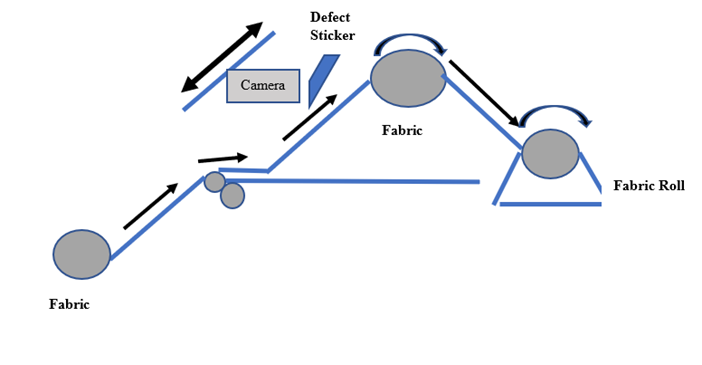
Fig.9 Automated Fabric Defect Detection
Future Research
Further research is warranted to enhance the robustness of the model by expanding the image dataset and incorporating a broader array of defect types for multi-classification purposes.
Additionally, more extensive research is needed to facilitate the deployment of this model within the textile industry. This would involve the implementation of infrared cameras and defect labelling machines to fully automate the fabric quality inspection process. Such endeavours would contribute to the comprehensive integration of the developed algorithm into practical industrial settings.
Acknowledgments
I extend a special thanks to Peiran Peng, the author of “Automatic Fabric Defect Detection Method Using PRAN-Net,” as well as to Kaggle for their invaluable support in facilitating the data collection process.
Conflict of interest statement
The authors have no conflict of interest to declare.
References
Agustianto, K. and Destarianto, P. (2019),’Imbalance Data Handling using Neighborhood Cleaning Rule (NCL) Sampling Method for Precision Student Modeling’, IEEE. pp.86-89.
doi:10.1109/ICOMITEE.2019.8921159
Almeida, T., Moutinho, F. and Matos-Carvalho, J., P. (2021) ‘Fabric Defect Detection with Deep Learning and False Negative Reduction’ IEEE Access, 2021, pp. 1-11. doi:10.1109/ACCESS.2021.3086028.
Brems, M. (2017), ‘A One-Stop Shop for Principal Component Analysis’, Towards Data Science, Available at: https://towardsdatascience.com/a-one-stop-shop-for-principal-component-analysis-5582fb7e0a9c
Chawla, V., N., Bowyer, K., W., Hall, L., O. and Kegelmeyer, W., P. (2002), ‘ SMOTE: Synthetic Minority Oversampling Technique’, Journal of Artificial Intelligence Research, 16(2), 321-357.
Chen, M. et al. (2022) ‘Improved faster R-CNN for fabric defect detection based on Gabor filter
with Genetic Algorithm optimization’ Computers in Industry, 134, pp. 103551.
doi: 10.1016/j.compind.2021.103551.
Cheng, L., Yi, J., Chen, A. and Zhang, Y. (2022), ‘Fabric Defect Detection Based on Separate Convolutional UNet’, Multimedia Tools and Applications, 82, pp. 3101-3122, https://doi.org/10.1007/s11042-022-13568-7
Chollet, F., et al. (2015). Keras. GitHub Repository. Retrieved from https://github.com/keras-team/keras
Duan, H., Wei, Y., Liu, P. and Yin, H. (2020), ‘A Novel Ensemble Framewok Based on K-Means and Resampling for Imbalanced Data’, Applied Sciences, 10, pp. 1-16. doi:10.3390/app10051684
Du, J. (2018), ‘Understanding of object detection based on CNN family and YOLO’, Journal of Physics: Conference Series. IOP Publishing, p. 012029. https://doi.org/10.1088/1742-6596/1004/1/012029.
Fan, H., Zhou, E. (2016), ‘Approaching human level facial landmark localization by deep learning’, Image Vis. Comput, 47, pp. 27–35. https://doi.org/10.1016/j.imavis.2015.11.004
Goodfellow, I., Bengio, Y., & Courville, A. (2016). Deep Learning. MIT Press.
Gowda. K., C. and Krishna, G. (1979), ‘The Condensed Nearest Neighbor rule using the concept of mutual nearest neighbor’, IEEE Transaction Theory, 25 (4), pp.488-490. Available at:
https://ieeexplore.ieee.org/stamp/stamp.jsp?tp=&arnumber=1056066
Han, H., Wang, W-Y. and Mao, B-H. (2005),’Borderline-SMOTE: A New Over-Sampling Method in Imbalanced Data Sets Learning’, ICIC , 878-887, doi:10.1007/11538059_91
He, H., Bai, Y., Garcia E. A. and Li, S. (2008),’ ADASYN: Adaptive Synthetic Sampling Approach for Imbalanced Learning’, International Joint Conference on Neural Networks,pp. 1322-1328, Available at:https://ieeexplore.ieee.org/stamp/stamp.jsp?tp=&arnumber=4633969
He, Y., Zhang, H., D., Huang, X., Y. and Tay, F., E., H. (2021), ‘Fabric Defect Detection based on Improved Faster RCNN’ International Journal of Artificial Intelligence& Applications, 12(4), pp.23–32. doi: 10.5121/ijaia.2021.12402.
Howarth, J. P., Zakharov, D. N., Megret, R. and Stach, E. A. (2020), ‘Understanding important features of deep learning models for segmentation of high-resolution transmission electron microscopy images’, npj Computational Materials, (2020)6:108, 9. doi: https://doi.org/10.1038/s41524-020-00363-x
Imbalanced Learn (n.d.a), ’SVMSMOTE’. Available at:
https://imbalanced-learn.org/stable/references/generated/imblearn.over_sampling.SVMSMOTE.html
Imbalanced Learn (n.d.b),’ClusterCentroids’. Available at: https://imbalanced-learn.org/stable/references/generated/imblearn.under_sampling.ClusterCentroids.html
Imbalanced Learn (n.d.c),’EditedNearestNeighbor’. Available at: https://imbalanced-learn.org/stable/references/generated/imblearn.under_sampling.EditedNearestNeighbours.html
Imbalanced Learn (n.d. d), ’RepeatedEditedNearestNeighbors’. Available at: https://imbalanced-learn.org/stable/references/generated/imblearn.under_sampling.RepeatedEditedNearestNeighbours.html
Imbalanced Learn (n.d.e),’AIIKNN’. Available at:
https://imbalanced-learn.org/stable/references/generated/imblearn.under_sampling.AllKNN.html
Imbalanced Learn (n.d.,f), ’Under-sampling’. Available at: https://imbalanced-learn.org/stable/under_sampling.html#edited-nearest-neighbors
Imbalanced Learn (n.d.h)’, Combination of Over- and Under-Sampling’. Available at: https://imbalanced-learn.org/stable/combine.html
Imbalanced Learn (n.d.i)’, ‘RandomOverSampler’. Available at: https://imbalanced-learn.org/stable/references/generated/imblearn.over_sampling.RandomOverSampler.html
Jing, J., Wang, Z., Rätsch, M. and Zhang, H. (2022), ‘Mobile-Unet: An efficient convolutional neural network for fabric defect detection’, Textile Research Journal, 92(1–2), pp. 30–42,
doi: 10.1177/0040517520928604.
kmeans-smote.readthedocs.io (no date),’kmeans_smote module’. Available at: https://kmeans-smote.readthedocs.io/en/latest
Kohavi, R. (1995). A study of cross-validation and bootstrap for accuracy estimation and model selection. In International Joint Conference on Artificial Intelligence (Vol. 14, No. 2, pp. 1137-1145). Morgan Kaufmann Publishers Inc.
Letteri, I., Cecco, A.D., Dyoub, A. and Penna, G. D. (2020), ‘A Novel Resampling Technique for Imbalanced Dataset Optimization’, Researchagte, pp. 1-23. Available at:
LeCun, Y., Bottou, L., Bengio, Y., & Haffner, P. (1998). Gradient-based learning applied to document recognition. Proceedings of the IEEE, 86(11), 2278-2324
Li, C., Li, J., J., Li, Y., He, L., Fu, X. and Chen, J. (2021), ‘Fabric Defect Detection in Textile Manufacturing: A Survey of the State of the Art’, Security and Communication Networks, 2021, pp. 1-13. doi: 10.1155/2021/9948808.
Lin, G., Liu, K., Xia, X. and Tan, R. (2023), ‘An Efficient and Intelligent Detection Method for Fabric Defects based on Improved YOLOv5’, Sensors, 23 (1), pp. 1-16, https://doi.org/10.3390/s23010097
Liu, Z., Zhang, C., Li, C., Ding, S., Dong, Y. and Huang, Y. (2019), ‘Fabric defect recognition using optimized neural networks’, Journal of Engineered Fibers and Fabrics, 14, pp. 1-10.
doi: 10.1177/1558925019897396.
Liu, Z., Liu, S., Li, C., Ding, S. and Dong, Y. (2018), ‘Fabric defects detection based on SSD’, ACM International Conference Proceeding Series, pp. 74–78. doi: 10.1145/3282286.3282300.
Luke, J. J., Joseph, R. and Balaji, M. (2019),’Impact of image size on accuracy and generalization of convolutional neural networks’, International Jouranl of Research and Analytical Reviews Ijrar, 6(1), pp.70-80, Available at: https://www.researchgate.net/publication/332241609.
Madhukar, B. (2020),’Using Near-Miss Algorithm For Imbalanced Datasets’, Developers Corner. Available at: https://analyticsindiamag.com/using-near-miss-algorithm-for-imbalanced-datasets/
Microsoft. (n.d.). Visual Studio Code – Code Editing. Redefined. Retrieved from https://code.visualstudio.com/
Minhas, M., S. and Zelek, J. (2020), ‘Defect detection using deep learning from minimal annotations’, VISIGRAPP 2020 – Proceedings of the 15th International Joint Conference on Computer Vision, Imaging and Computer Graphics Theory and Applications, 4, pp. 506–513. doi: 10.5220/0009168005060513
Pahren, L., Thomas, P., Jia, X. and Lee, J. (2022),’A Novel Method in Intelligent Synthetic Data Creation for Machine Learning-based Manufacturing Quality Control’, IFAC PapersOnline, 55-19(2022), pp. 73-78. DOI:10.1016/j.ifacol.2022.09.186.
Pathirana, P. (2020), ‘Fabric stain dataset’, Kaggle, Available at: https://www.kaggle.com/datasets/priemshpathirana/fabric-stain-dataset
Prakash, S., Berry, D., P., Roantree, M., Onibonoje, O., Gualano, L., Scriney, M. and McCarren, A. (2021),” Using artificial intelligence to automate meat cut identification from the semimembranosus muscle on beef boning lines”, Journal of Animal Science, 99 (12), 1-13, https://doi.org/10.1093/jas/skab319
Peng, P., Wang, Y., Hao, C., Zhu, Z., Liu, T. and Zhou, W. (2020) ‘Automatic fabric defect detection method using pran-net’ Applied Sciences (Switzerland), 10 (23), pp. 1–13.https://dl.acm.org/doi/abs/10.1016/j.compind.2021.103551.
Ranathunga, S. (2020), ‘Fabric defect dataset’, Kaggle, Available at: https://www.kaggle.com/datasets/rmshashi/fabric-defect-dataset
Rasheed, A., Zafar, B., Rasheed, A., Ali, N., Sajid, M., Dar, S. H., Habib, U., Shehryar, T., Mahmood, M., T. (2020) ‘Fabric Defect Detection Using Computer Vision Techniques: A Comprehensive Review’ Hindawi Mathematical Problems in Engineering, 2020, pp. 1-24, https://doi.org/10.1155/2020/8189403
Ringner, M. (2008)’what is principal component analysis’,Nature Biotechnology,26(3), pp.303-304, Available at: http://146.6.100.192/users/BCH339N_2018/NBT_primer_PCA.pdf
Rukundo, O. (2021), ‘ Effects of image size on Deep Learning’, Arxiv, pp.19, doi:10.48550/arXiv.2101.11508
Silvestre-Blanes, J., Albero-Albero, T., Miralles, I., Pérez-Llorens, R. and Moreno, J. (2019), ‘ Aitex Fabric Image Database’, Aitex, Available at: https://www.aitex.es/afid/
Sabottke, C., E. and Spieler, B. M. (2019) ‘The Effect of Image Resolution on Deep Learning in Radiography’, Radiology: Artificial Intelligence, 2(1), pp.1-7,
Available at: https://doi.org/10.1148/ryai.2019190015
Sisters, Li. (2020),’Instance Hardness Threshold: An Undersampling Method to Tackle Imbalanced Classification Problems’, Towards Data Science. Available at: https://towardsdatascience.com/instance-hardness-threshold-an-undersampling-method-to-tackle-imbalanced-classification-problems 6d80f91f0581#:~:text=Instance%20Hardness%20Threshold%20(IHT)%20is,be%20removed%20from%20the%20dataset.
TensorFlow. (n.d.). Retrieved from https://www.tensorflow.org
Thambawita, V., Strumke, I., Hicks, S. A., Halvorsen, P., Parasa, S. and Riegler, M. A. (2021), ‘Impact of Image Resolution on Deep Learning Performance in Endoscopy Image Classification: An Experimental Study Using a Large Dataset of Endoscopic Images’ , National Library of Medicine,11(12):2183, doi: 10.3390/diagnostics11122183
Vladimir, P. (2020),’Handling imbalanced dataset in image classification’, Analytics Vidhya. Available at: Handling imbalanced dataset in image classification | by Privalov Vladimir | Analytics Vidhya | Medium
Viadinugroho, R. A.A. (2021),’Imbalanced Classification in Python: SMOTE-Tomek Links Method’, TowardsData Science, Available at: https://towardsdatascience.com/imbalanced-classification-in-python-smote-tomek-links-method-6e48dfe69bbc
Wang, Z. and Jing, J. (2020) ‘Pixel-Wise Fabric Defect Detection by CNNs without Labeled Training Data’, IEEE Access, 8, pp. 161317–161325. doi: 10.1109/ACCESS.2020.3021189.
Wallelign, S., Polceanu, M., Buche, C., (2018), ‘Soybean plant disease identification using convolutional neural network’, The Thirty-First International Flairs Conference.
Wei, B., Hao, K., Tang, X., S. and Ren, L. (2019) ‘Fabric defect detection based on faster RCNN’ in Advances in Intelligent Systems and Computing, 849, pp. 45–51. doi: 10.1007/978-3-319-99695-0_6.
Wilson, D., L. (1972),’Asymptotic Properties of Nearest Neighbor Rules Using Edited Data’, IEEE Transactions of Systems, Man and Cybernetics,2 (3), 408-421. DOI: 10.1109/TSMC.1972.4309137
Yamashita, R., Nishio, M., Do, R., K., G. and Togasi, K. (2018), ‘Convolutional neural networks: an overview and application in radiology’, SpringerOpen,
Available at: https://insightsimaging.springeropen.com/articles/10.1007/s13244-018-0639-9
Zhao, Y., Hao, K., He, H., Tang, X. and Wei, B. (2019) ‘A visual long-short-term memory based integrated CNN model for fabric defect image classification’ Neurocomputing, 380, pp. 259–270. doi: 10.1016/j.neucom.2019.10.067.
Zhao,S., Yin, L., Zhang, J., Wang, J. and Zhong, R. (2020) ‘Real-time fabric defect detection based on multi-scale convolutional neural network’ IET Collaborative Intelligent Manufacturing, 2(4), pp. 189–196. doi:10.1049/IET-CIM.2020.0062.
Zhang, H., Zhang, L., Li, P. and Gu, D. (2018)’Yarn-dyed Fabric Defect Detection with YOLOV2 Based on Deep Convolution Neural Networks’, IEEE 7th Data Driven Control and Learning Systems Conference, pp. 170-174. doi: 10.1109/DDCLS.2018.8516094
Appendix A- Sampling Techniques (PCA, Confusion Matrix)
Undersampling Techniques
AIKNN